Berkeley Lab Internship · Braedyn Thompson

Overview01

-24%RMSE vs persistencebest target

3yrof XCache traffic logsEDA + forecasting

Alltargets beat baselineevery horizon

Multihorizon forecaststuned lookback windows

XCache is a data cache layer for large scientific workflows. If you know traffic will spike, you can provision for it. If you miss the spike, everything downstream slows down.

My work had two halves. One was building a forecaster that beats the hard-to-beat naive baseline. The other was finding out, with evidence, how predictable the peaks are at all, so the team designs features and models around a real ceiling instead of chasing it.

01
Implemented PatchTST (PyTorch / neuralforecast) for multivariate time-series forecasting of cache-traffic signals across multiple horizons, tuning lookback windows and beating a persistence baseline on all targets by up to 24% RMSE.
02
Exposed the ceiling on peak-load predictability and guided feature and model design by building reproducible Pandas EDA pipelines over 3 years of XCache traffic logs. I visualized seasonality, change-points and right-skewed peaks with Matplotlib, Seaborn and Plotly, and used rolling cross-validation to show that models under-predict rare peaks.

Forecasting with PatchTST02

PatchTST treats a time series the way a vision transformer treats an image. It cuts the lookback window into short patches, turns each patch into a token, and lets a Transformer attend across patches. Each channel is handled independently with shared weights. Patching keeps local shape (a ramp, a burst) intact inside one token and cuts the sequence length the attention has to cover.

SchematicHow PatchTST sees a lookback window: patches become tokens, a channel-independent Transformer encodes them, and heads emit forecasts at several horizons. Schematic only, not real data.

The baseline that's hard to beat

For traffic, "tomorrow looks like today" (persistence) is a strong baseline. Most of the signal is momentum and daily rhythm. A model that can't beat persistence on every horizon isn't worth deploying, so persistence was the bar for every target.

Persistence is hard to beat. PatchTST beat it on every target.

FigurePersistence indexed to 100. PatchTST beat it on every target; the largest margin was 24% lower RMSE.

What I tuned

Lookback window length per horizon. Longer windows capture weekly structure, while shorter ones adapt faster to change-points.
Forecast horizons from short to long, with a separate evaluation for each so a good short horizon can't hide a weak long one.
Evaluation that is always walk-forward. No fold ever trains on data that comes after its test window.

Daily hit_size, actual vs PatchTST — **Figure**Daily hit_size (TB) over the test period: actual vs. PatchTST. The forecast tracks the everyday level and rhythm, but the rare spikes (some above 200 TB) are far above the prediction.

Lookback depends on the horizon

The best lookback window isn't fixed. At 1-day and 7-day horizons a ~100-day lookback wins, which reflects real seasonality. At a 30-day horizon that advantage disappears:

At 30 days out, short lookbacks win. 100–300 days never does.

Feature	3	7	14	28	40	60	80	100	120	150	200	300
access_count	11,641	11,858	12,915	13,219	12,774	12,601	12,150	11,917	11,803	12,506	12,327	12,898
access_size	28.51	29.52	31.47	33.36	32.11	33.08	32.01	32.18	33.45	33.44	32.15	34.23
hit_count	10,708	10,880	11,358	12,264	11,815	11,669	11,010	10,955	10,988	11,745	11,786	12,117
hit_size	27.95	29.02	30.64	32.72	31.46	32.59	31.36	31.56	32.90	32.93	31.85	33.75
miss_count	1,475	1,444	1,677	1,300	1,768	1,704	1,697	1,879	1,737	2,030	1,896	2,640
miss_size	0.860	0.785	1.030	0.715	0.956	0.962	0.936	1.009	1.030	1.049	1.080	1.673

RMSE by lookback window (days) at a 30-day forecast horizon, per feature; lower is better and the best per feature is highlighted.

Long lookback doesn't help at 30 days. A 3-day lookback wins on 4 of the 6 features and 28 days wins the other 2; 100–300-day lookbacks are never the best. The ~100-day seasonal advantage seen at the 1- and 7-day horizons doesn't carry over to a 30-day forecast. The shape of the error curve does hint that a lookback around 120 days could do better, which is worth testing next.

So a longer lookback is always better?

Not at a 30-day horizon. A 3-day lookback wins 4 of the 6 features, and 100+ days never wins.

But the 100-day window wins at 1 and 7 days?

Right. The seasonal advantage just doesn't carry out to 30 days.

EDA & the predictability ceiling03

Before modelling, I built reproducible Pandas pipelines over three years of XCache logs: loading, cleaning, resampling, and a fixed set of diagnostic views that rerun end to end on new data.

SeasonalityDaily and weekly rhythm in request volume, which is what persistence and the model both exploit.

Change-pointsRegime shifts where the level or variance of traffic jumps, so a window from before is misleading after.

Right-skewed peaksMost hours are ordinary and a few are extreme. The tail is what operations care about most.

Rolling CVWalk-forward folds that show where errors concentrate over time.

SchematicRolling-origin cross-validation: each fold trains only on the past and validates on the next block, which mirrors how the model would actually be used.

Walk-forward only: no fold ever peeks at the future.

The finding: a ceiling on peaks

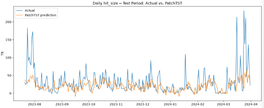
Across folds the models track the baseline load well but systematically under-predict rare peaks. Peaks are right-skewed, infrequent, and often not foreshadowed in the lookback window, so a model trained to minimize average error learns to hedge toward the typical level. That changed the question the team asked. Instead of "which architecture predicts peaks?", it became "what signal would make peaks predictable?", and that question drives feature design.

Does the loss function fix it?

One natural fix is to change what the model is trained to minimise. I compared five losses, from the softest (MAE) through Huber at three thresholds to the strictest (MSE), on hit_size with a 100-day lookback at a 1-day horizon.

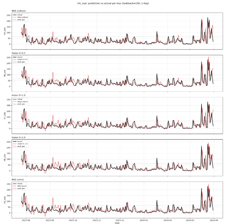
Prediction vs actual for five loss functions — **Figure**hit_size, prediction vs. actual for five training losses (MAE, Huber δ = 0.5 / 1.0 / 2.0, MSE), lookback 100, 1-day horizon. The shaded areas are the peak gap: under every loss the largest spikes are still under-predicted.

Five losses, same story: the biggest spikes stay under-predicted.